
INTRODUCTION
Fractures result from rock brittle failure in the Earth’s crust. They control the physiography of many spectacular landforms and play an essential role in the transport of fluids (e.g., Pollard & Aydin, 1988). The spatial arrangement of fractures gives rise to a fracture network, wherein the position, orientation, and interrelationships among individual fractures are mapped in 2D or 3D space (Gillespie et al., 1993; Odling et al., 1999; Marrett et al., 2018; Laubach et al., 2018; Peacock et al., 2018; Sanderson & Peacock, 2019). Generally, in fracture patterns, it is possible to recognise a master set with regular form, spacing, and orientation (also referred to as systematic joints) and one or more cross-joint sets that are irregular in form, spacing, and orientation, interrupting the master set (also referred to as unsystematic joints). Moreover, fracture patterns can be orthogonal, polygonal, and conjugated depending on the spatial relationships between the fractures (Bai et al., 2002; Correa et al., 2022; Fossen, 2016). Extrapolation of fracture properties (length, orientation, and spatial distribution) across observation scales is essential for reconstructing the deformation history of an area (Cawood et al., 2023; Ceccato et al., 2022; Menegoni et al., 2022b). In addition, their presence controls some rock characteristics, such as secondary porosity, permeability (Ceccato et al., 2021; Wang et al., 2018), and rock mass integrity (e.g., Palmstrom, 1996).
Studying how fractures are arranged on outcrops and how lithology varies spatially helps predict their distribution in the subsurface and how they influence secondary porosity and rock permeability (e.g., Dichiarante et al., 2020; Watkins et al., 2018, 2019), which are critical parameters for fluid migration (e.g., Guerriero et al., 2013; Malinouskaya et al., 2014; Panara et al., 2023; Moretti, 1998) or underground storage capacity for CO2 (Damen et al., 2006; Fedorik et al., 2023; Rizzo et al., 2024) and clean energy carriers (e.g., hydrogen Heinemann et al., 2021).
Before modern technology’s advent, fracture distribution was analysed by studying rocks in the field using a compass and measuring tape. Additionally, remote methods, such as photogrammetry from aircraft, were utilised for this purpose. However, with the advent of drones and smartphones, attention has shifted to computerised methods that can save time and handle a large amount of data (Ovaskainen et al., 2022; Salvini et al., 2016; Smeraglia et al., 2021; Tavani et al., 2022). Mercuri et al. 2023 showed how manually or semi-automatically interpreted satellite and aerial images can be used in characterising fracture networks but that the appropriate scale of interpretation is crucial because the resolution of the dataset strongly influences the fracture network (Bour et al., 2002; Cawood et al., 2023; Ceccato et al., 2022; Espejel et al., 2020). Fracture network characterisation is not limited to satellite and aerial imagery. It can be applied to wellbore data (e.g., Aliverti et al., 2003; Yasin et al., 2022; Ozkaya and Mattner, 2003; Petrik et al., 2023) and more recently, it has been applied to reflection seismic data, despite its lower resolution, with interesting results. (e.g., Osagiede et al., 2023; Crutchley et al., 2023).
Structural geologists use statistics to identify trends, understand mean(s) and dispersion in datasets, test hypotheses, evaluate implicit assumptions, and communicate the confidence of our interpretations to peers (Roberts et al., 2019). For that, different authors developed software that can automatically (Alzubaidi et al., 2022; Cao et al., 2017; Prabhakaran et al., 2019) or semi-automatically (Figorito et al., 2014; Lee et al., 2022; Thiele et al., 2017; Vasuki et al., 2013) digitise fractures from the 2D model of an outcrop. Digitising fractures in a 2D or 3D Digital Outcrop Model (DOM) is the first step in Discrete Fracture Network (DFN) development (Giuffrida et al., 2020; Massaro et al., 2019; Pereira et al., 2024; Smeraglia et al., 2021). Different softwares have been developed to perform statistical analysis of fracture patterns and extract attributes from digitised fractures of an outcrop.
For instance, DigiFract is a Python-based software that digitises fractures on a 2D outcrop and performs analysis with rose diagrams (Hardebol & Bertotti, 2013). FracPaQ is a MATLAB toolbox for quantifying fracturing patterns in 2D from digital data in various formats and creating fracture density maps (Healy et al., 2017). NetworkGT is a GIS toolbox consisting of 18 tools for analysing fracture patterns and their topology (Nyberg et al., 2018). FraNEP is a software developed in Visual Basic to manage fracture data and provide a statistical characterisation of fracture networks by correcting censoring biases (Zeeb et al., 2013a). DICE is an open-source application for quantitatively characterising fractures within a 3D DOM of a rock mass (Menegoni et al., 2022a).
Previous software or tools involved complex data preparation or handling methods that returned unwieldy results and needed help controlling where to place the scanning areas. We developed a new Python-based Fracture Analyser (FA) software to try to overcome these limitations. It does not require complex data preparation; it allows for easy result handling and enables multiple analyses on the same dataset with control over the positioning of the scan area. FA can derive the attributes from 2D digital fracture traces, and, in the future, it will implement new functionalities (e.g., fracture topology, branches, and nodes).
What convinced the authors to develop FA, rather than using existing tools, was the need to consolidate all the functions listed below within a single software platform usable with basic knowledge of Python and graphics software: The ability to produce a well-organised output file, where each line corresponds to a fracture and the associated features are systematically arranged in columns; the simplification of scale management by integrating it as a graphical element within the input file; the improvement of quality control through the identification of unprocessed fractures by highlighting them; the ability to rapidly process large files (even over 30,000 fractures) within seconds; the flexibility to perform both scan area and scanline analyses with control over their positioning; and the output of the scanline orientation and distance between fractures in a single file, facilitating the calculation of their real spacing (Terzaghi, 1965). Therefore, it is possible to perform numerous analyses (e.g., scanline Priest & Hudson, 1981 and scan area Dershowitz & Herda, 1992) with control over the positioning of the scanline or scan area to obtain new fracture attributes. The most crucial 2D fracture attributes, such as their length, orientation, and relative position in space, can all be obtained using FA (Tab.1). Of course, field data acquisition can provide additional attributes, such as fracture aperture, type of infill, and real attitude, which can subsequently be incorporated into the static geological model. Therefore, FA is not intended to be a definitive and comprehensive tool for analysing fracture patterns without ground truthing or fieldwork but rather a simple toolbox to facilitate digital analysis of fracture patterns in a wide range of scale observations.
| Attribute | Unit | Comments | Function | ||
|---|---|---|---|---|---|
| Fracture list | Scanline | Scan area | |||
| Trace abundance | n/a | ✓ | ✓ | ✓ | |
| Trace length | chosen by user | ✓ | ✓ | ✓ | |
| Distance from origin | chosen by user | The origin is the starting point of the scanline | ✓ | ||
| Apparent spacing | chosen by user | The distance is calculated between two adjacent fracture traces along the same scanline | ✓ | ||
| Density, P20 | X-2 | ✓ | |||
| Intensity, P21 | X-1 | ✓ | |||
| Trace orientation | Degrees | ✓ | ✓ | ✓ | |
The acquisition of fractures to be processed with FA can be performed by using the methodology chosen by the user: automatic, semi-automatic, or manual. It’s important to note that the accuracy and quality of the dataset directly impact the precision of FA output results. In this work, fractures were digitised manually through Adobe Illustrator for greater accuracy.
We have accepted the challenge proposed by Bonnet et al. (2001), in their section 8.6 “Future Research”) by developing a software capable of effectively deriving I) the spatial relationships among fractures in a population and II) orientation and position simultaneously.
It is well known that 2D digital fracture data are subject to numerous errors and biases, such as truncation, censoring, f-bias, the “cut effect”, occlusion and orientation bias (Sturzenegger & Stead, 2009; Zeeb et al., 2013b and references therein). Truncation refers to the under-representation of smaller fractures due to the resolution limits of the sampling method (Bonnet et al., 2001). Censoring is when longer fractures are not accurately sampled due to a small sample window, so those lengths are lost from the analysis. Sturzenegger et al. (2007) points out that censoring can occur because only a tiny part of the discontinuity surface is visible on a rock face, while most of it is hidden within the rock mass or has been eroded. In scanline surveys, the censoring bias is referred to as f-bias by Priest (2004). The “cut effect” is the geometric error caused by the intersection of 3D fracture planes with the 2D plane of the analysed outcrop. Occlusion bias refers to the inability to sample a complete rock face from a single position, resulting in partial visibility of fractures. Occlusion occurs when certain portions of a rock face are obstructed and inaccessible for sampling due to protruding features. It is widely recognised that the orientation bias can influence discontinuity measurements obtained from conventional scanlines (Terzaghi, 1965). The orientation bias can be vertical or horizontal and occurs when dealing with surfaces (discontinuities) that are sub-parallel to the camera/scanner’s line of sight, making them not visible to the camera/scanner. Fractures exist on a wide range of scales, from micro to macro scale, and it is known that throughout this scale range, they significantly affect Earth’s crust processes, including fluid flow and rock strength (Bonnet et al., 2001; Ceccato et al., 2022; Dichiarante et al., 2020; McCaffrey et al., 2020). An example of a complete set of observational scales includes samples, outcrops, UAV imagery, satellite imagery, and regional analysis.
The input data consists of a scalable vector graphic file (SVG) containing digital fracture traces and polygons to analyse the region of interest. The software outputs attributes of individual fractures, characteristics for the entire pattern, and attributes for a single fracture set. With all these attributes, it is possible to perform a statistical analysis of fracture patterns (Roberts et al., 2019). The software is currently limited to 2D fracture pattern analysis.
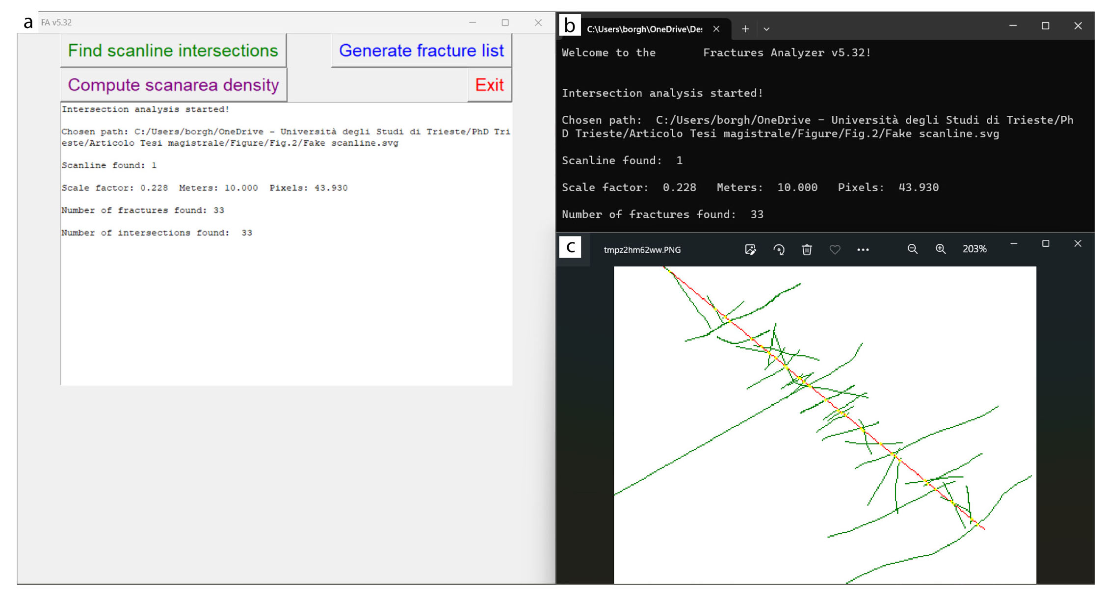
FA is an open-source software developed in Python that provides a simple and immediate tool for analysing fracture patterns (Fig. 1). It allows working with large amounts of data and provides the results in a simple format (.txt) for further processing with other softwares.
- Fracture Analyser user interface, function selection buttons, and short report (a), a brief report of the analysis performed (b), and the output image of the analysis performed (c).
The abundance of fractures in a rock mass is described by fracture intensity. It is generally defined using the Pij system introduced by Dershowitz & Einstein (1988), as well as Dershowitz & Herda (1992). The letter P stands for persistence, i for area dimensionality, and j for fracture dimension. Measurements can be carried out in one dimension (1D) scanline (i=1), two-dimension (2D) scan area (i=2), three-dimension (3D) volume (i=3), while fractures can be characterised by their abundance (j=0), length (j=1), area (j=2) or volume (j=3). For instance, P20 represents the number of fractures (j=0) per unit area (i=2). P11, P22, and P33 are dimensionless and represent porosity, P20 (m-2) and P30 (m-3) represent the frequency or density of fracturing, while intensity is represented by P10, P21, P32 (m-1). Fracture intensity is generally measured by 1D or 2D methods (Priest & Hudson, 1981; Mauldon et al., 2001; Rohrbaugh et al., 2002; Ortega et al., 2006; Watkins et al., 2015). The Pij classification system allows to compare the fracture intensity between two or more rock masses, and the most common sampling methods are for 1D the scanline method (e.g., Peacock et al., 2003; Priest, 1993; Priest & Hudson, 1981) and for 2D the scan area method (e.g., Dershowitz & Herda, 1992; Mauldon et al., 2001; Rohrbaugh et al., 2002). In this study, P10, the fracturing density per unit length, P20 and P21, respectively, density and intensity of fracturing per unit area are calculated using FA.
Natural cases
This study used a multiscale approach to digitise and extract fracture attributes from the Rosario pavement and Muggia sub-vertical wall, covering a scale range from more than 50 m to less than 5 m. We selected these outcrops because they represent ideal candidates for FA analysis. For their exceptional exposure, given that they do not show significant topographical variations, fractures therein are well exposed, and the possibility of using FA on both pavements and wall outcrops is shown.
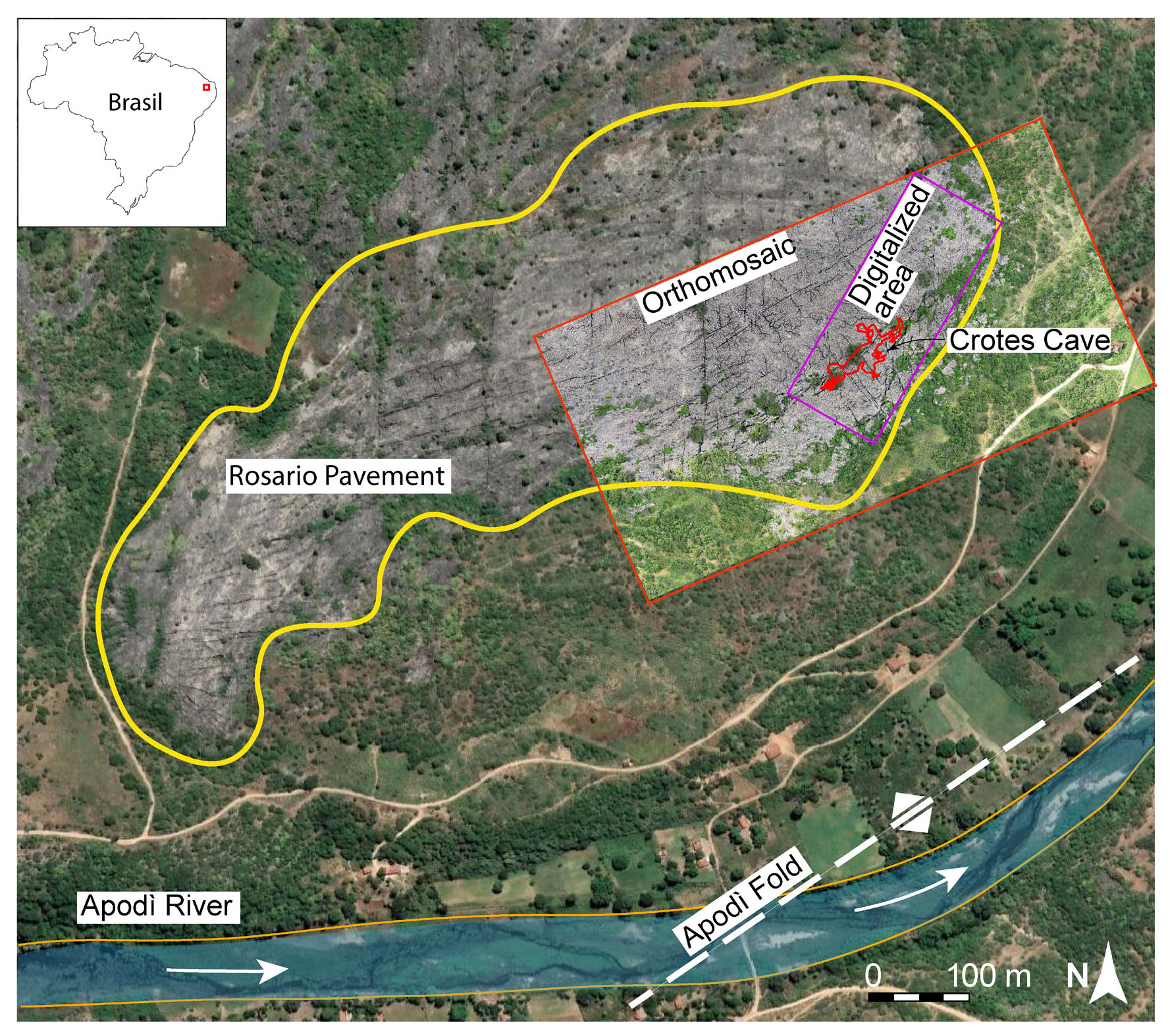
The Rosario pavement (Fig. 2) is composed of limestone of the Cretaceous Jandaira formation, is exposed along the bank of the Apodì River about 6 km north of Felipe Guerra (Rio Grande do Norte, BR), and is approximately 0.5 km2 in area. In this area the ground level undulates between 59 m and 61 m above sea level. The Jandaira formation is a post-rift unit of the Potiguar Basin and was deposited from the Turonian (93.9 Ma) to the Campanian (72.1 Ma). The exposed limestone sequence mainly comprises mudstones, peloidal packstones, and grainstones (Santos Filho et al., 2015). Jandaíra carbonates are gently dipping (<5°) beds that dip to the north. Subsequently, these carbonates were dissected by extensional faults associated with the South Atlantic opening (De Matos, 1992; Pessoa Neto et al., 2007). The recent work of Bagni et al. (2020) describes the presence of a mild anticlinal fold, called Apodì Fold (Fig. 2), that affects the Jandaira Formation limestone. The fold axis is NE-trending and positioned on the Apodì River’s course. In the Rosario pavements, the Crotes Cave (5° 33’ 38.9 “S; 37° 39’ 32.1 “W) (Fig. 2) develops a few metres below ground level and extends downward for 25 m and horizontally for ~125 m. The cave has a prevalent NE-SW direction (N50°E). Both open modes of fractures, veins, and joints are present in the outcrop (Bezerra et al., 2020). Moreover, the Rosario pavement is considered an analogue of the reservoirs present in the offshore portion of the Potiguar Basin.
- Satellite view of the Rosario outcrop, where the yellow line outlines the study area, the red line is the high-resolution orthomosaic, and the purple line is the digitised area with the Crotes cave in red.
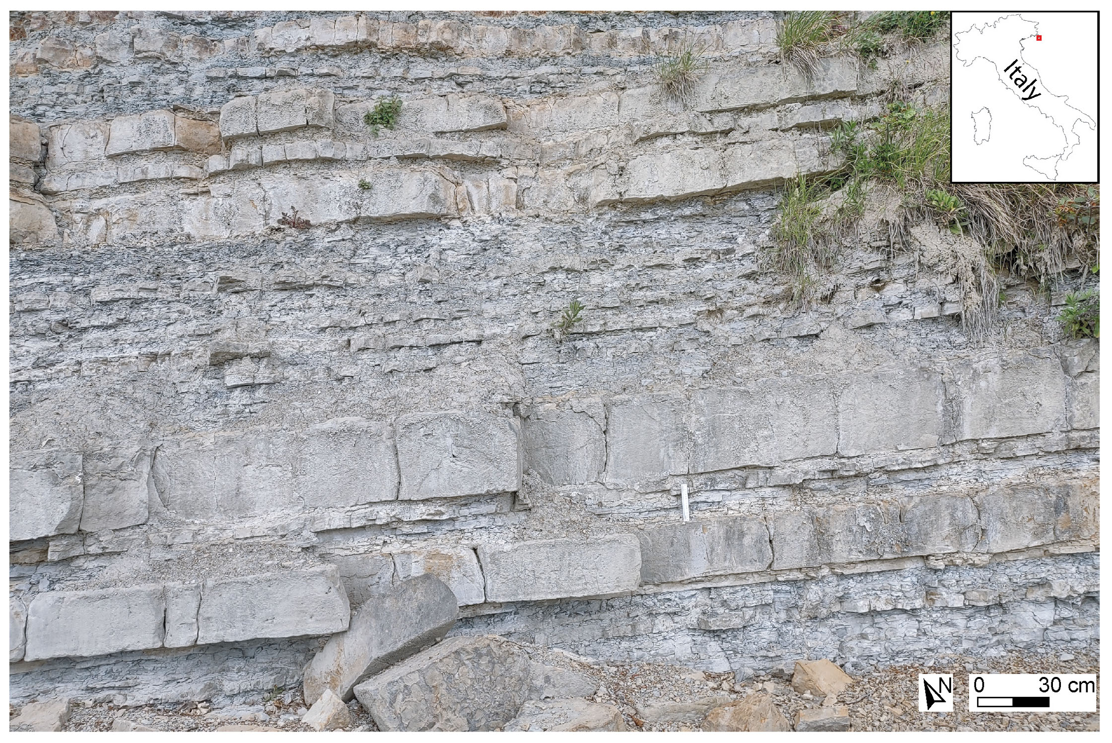
The Muggia outcrop is a sub-vertical wall composed of sandstone layers related to the Flysch of the Trieste formation, exposed on a seashore cliff near the city of Muggia (Friuli-Venezia Giulia, North-East Italy) (Fig. 3). This sandstone interval, deposited during the Middle Eocene (~ 41 Ma), displays a dip angle of 20° toward north and is affected by numerous fractures, faults, and folds due to the compressional phases associated with the Alpine orogeny (Dinaric phase, - Oligocene age) (Carulli, 2011) and belongs to the external Dinarides (Poljak et al., 2000).
- Muggia sub-vertical outcrop where well-exposed fractures can be seen in the thicker layers.
PROGRAM DESCRIPTION
FA is an open-source code, and it was developed to generate fracture pattern attributes where the user controls the analysis area and the scale. The source code, test files, and the user manual are available from GitHub (https://github.com/LorenzoBorghini/FA). The data used in this research are available to the first author upon request. FA is available as a Python extension (.py) for users and developers who want to improve it. Before running FA, you must install the latest version of Python (3.12.0 or later versions) and one graphics library (i.e., Pillow library). The software is written in Python for the simplicity of writing and the possibility of quickly implementing further functions and add-ons.
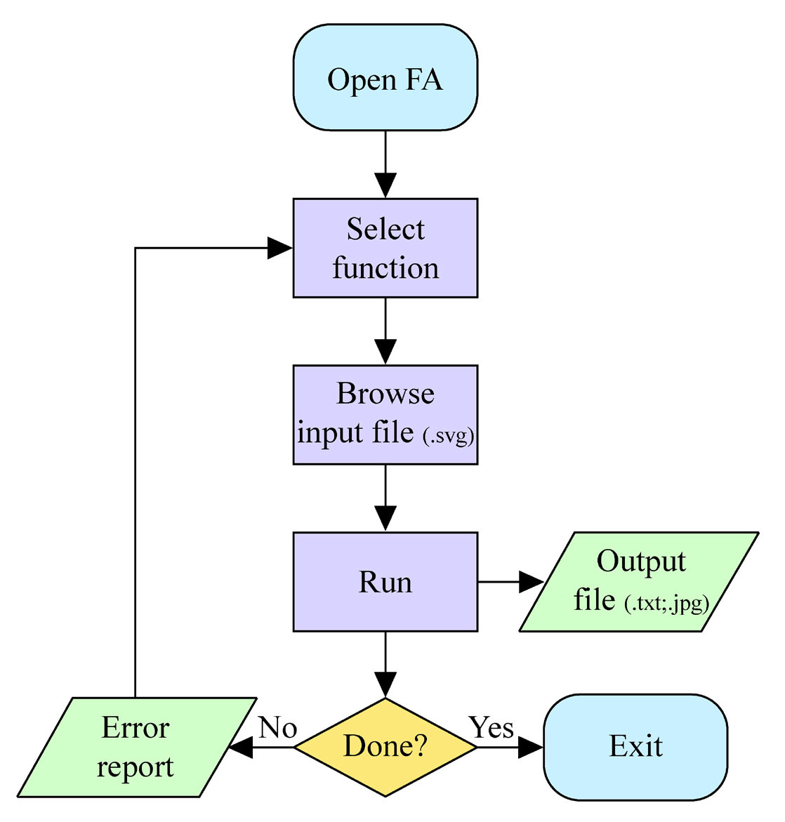
FA is currently capable of performing three types of fracture patterns analyses (Tab. 1 functions section), providing five parameters for each individual fracture (e.g., number, length, orientation, distance from origin, and apparent spacing) and three for the entire fracture dataset (e.g., apparent spacing, fracture density P20, and intensity P21). The flow chart of FA is shown in Fig. 4. Below is a list of the functions of FA:
- linear scanline
- convex polygon scan area
- list of all fractures and their attributes.
- Flowchart of FA operation.
Input file format
FA currently accepts only appropriately constructed and named “Scalable Vector Graphics” (.SVG) files. The dataset examples in this study were created using Adobe Illustrator, the only software currently able to generate a fully FA-compatible SVG. The graphic file (.SVG) must have a layer for the fractures (to be chimed compulsorily “fractures”), a layer for the scale (to be chimed compulsorily “scale”), and a layer for the scanline or scan area (to be chimed compulsorily “scanline” or “scanarea”, respectively). In the “scale” layer, a segment and a number indicating its real length are placed in a unit of measurement at the user’s preference. The layer containing the fractures must contain only vectors of the digitised fractures, and the layer of a scanline or scan area must contain only a vector geometry (e.g., the “scanline” layer must contain only a line, and the “scanarea” layer must contain only a closed polygon).
Internal data structure and calculated quantities
FA quantifies fracture attributes such as number, length, spatial orientation, spatial position, the angle between scanline and fracture, apparent spacing, density (P20), and intensity (P21), as described in Dershowitz & Herda (1992). These attributes and their units are listed in Tab. 1.
When a valid file is fed to FA, the software extrapolates fracture lengths using an equation based on the end node coordinates (x and y). The same process is repeated during scanline analysis to calculate the distance of each fracture from the origin and determine its apparent spacing. Fracture density and intensity are calculated using circular scan areas or other concave polygonal geometry (e.g., square, rectangle, or triangle).
The distance between fractures along a scanline is returned as an apparent spacing. However, if the input dataset belongs to the same fracture set and the scanline is orthogonal to the fractures, the apparent spacing should be understood as the real spacing. The apparent spacing can be easily corrected using the Terzaghi correction (Peacock et al., 2003; Terzaghi, 1965) since FA provides both the spatial orientation of the scanline and the fractures.
When FA is launched, users can choose the type of analysis they wish to perform on the fractures, import the correctly compiled input file (.SVG), and automatically return the output file. The output file for each analysis is created in the same folder as the input file and is named inputfilename_analisys. It is a text file (.txt) divided into columns subdivided by tabs, and each line belongs to a specific fracture. The user chooses the unit of measurement for all length attributes when he creates the “scale” layer in the graphic software and inserts the numerical scale reference value. The angles are expressed in decimal degrees with respect to the Y axis, which is assumed to be the real north.
APPROACHES AND METHODS
Due to 2D input data and software limits, FA assumes the input fracture traces to lie on a flat 2D surface, such that no topographical geometry correction is necessary. Currently, FA cannot process curvilinear fracture traces, so it is necessary to simplify them (i.e., polyline) through some software simplification tools. Despite the stated assumptions, the results produced by FA are to be considered reliable and sound. During the analysis, FA takes into account the entire fracture trace, and the direction (i.e., strike) of the polyline fracture traces is calculated for the line passing through the first and last points of the trace. This method is statistically accurate since fractures intersecting a plane can often be simplified as straight lines. The length and all other spatial attributes are calculated from simple geometric calculations performed on the coordinates of the track points.
The number of fractures in the dataset is the starting data from which all subsequent processing can be done, and FA considers each fracture trace as a single fracture, just as it would happen in the field.
The azimuthal orientation of fracture traces in FA can be calculated only if the inserted fracture traces belong to a pavement outcrop. The Y axis is assumed to be true north, and all orientations are calculated clockwise from 0° to 180. Analysis of walls is still possible; however, the calculated orientation parameter should be excluded.
The length of the fractures is essential to draw structural geology considerations, and it is calculated using a scaling factor entered when constructing the SVG file. The unit of measurement is the user’s choice and is the same as that of the scale (e.g., if the scale is in metres, the length of the fractures in the output file will be given in metres).
When analysing a linear scanline, FA returns the number and length of fractures with which P10 (Dershowitz & Herda, 1992) can be calculated, where P10 is the density of fractures per unit length (number of fractures per unit length) (Dershowitz & Herda, 1992).
FA can analyse linear scanlines to obtain the apparent spacing between two fracture traces. Having the apparent spacing returned by FA, it is possible to calculate the real spacing between fractures belonging to the same set using the Terzaghi correction (Peacock et al., 2003; Terzaghi, 1965):
Realspacing=apparentspacing·(ϑsl·ϑfs)[m]Where ϑsl and ϑfs are the azimuths, respectively, of the scanline and the fracture set with respect to the north, the real spacing is the orthogonal distance between fractures of the same set, and the apparent spacing is the non-orthogonal distance between fractures. Using the real spacing of fractures belonging to one set along one or more scanlines, it is possible to perform statistical analyses on the spatial distribution of fractures by calculating the coefficient of variation Cv, the Fractures Spacing Ratio (FSR) in individual beds (Gross, 1993) and the Fractures Spacing Index (FSI) for bed’s packages (Narr & Suppe, 1991). The Cv corresponds to the ratio of standard deviation to mean spacing. Cv values < 1.0 characterise an anti-clustered distribution, while Cv values > 1.0 indicate a clustered distribution of fractures (Gillespie et al., 1993). The FSR and FSI indexes are indicators of fracture density. They can analyse mechanical stratigraphy on a sub-vertical outcrop, where FSR refers to a single layer and FSI refers to a layered rock mass. The FSR corresponds to the ratio of layer thickness to fracture spacing. The slope of the linear interpolation of the various FSRs corresponds to the FSI.
The scan area analysis returns the values of P20 and P21, which are the density and intensity of fracturing per unit area, respectively (Dershowitz & Herda, 1992).
P20=Nf/A[m−2]andP21=ΣLf/A[m−1]where Nf is the number of fractures, A is the area of the scan area, and ΣLf is the fracture trace length sum. These parameters are obtained from a scan area positioned by the user at the desired location above the digitised fractures dataset.
The data obtained from the two outcrops were then processed using the Moving Average Rose Diagram (MARD) (Munro & Blenkisop, 2012) for the orientation’s statistical analysis and Microsoft Excel for other statistical analyses.
Digital acquisition of outcrops
For the Rosario pavement outcrop we used a standard drone DJI Phantom 4 pro UAV with a 24 mm camera lens, recording images at 21 megapixels, to construct a high-resolution photogrammetric survey. The drone was flown in a regular grid pattern at a constant altitude of 60 m above local ground level. The digital photographs were processed to build an orthomosaic (Fig. 2) of the whole area, including lens correction. The final orthomosaic (Fig. 2) has a ground resolution of about 0.04 m/pixel and was georeferenced and scaled using the integrated GPS information of the drone.
For the Muggia sub-vertical outcrop, we used a standard digital camera with a resolution of 48 megapixels. The image (Fig. 3), with a ground resolution of about 0.0005 m/pixel, was taken orthogonal to the outcrop at a distance of 7 m.
RESULTS AND APPLICATIONS
This section describes the practical applications and outputs from FA exemplified by the Rosario (Fig. 5) and Muggia (Fig. 9a) datasets. In both cases, digital fractures were traced at multiple scales of observation.
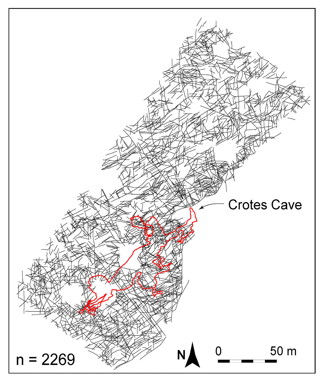
- Dataset of digitised fractures on Rosario outcrop in black and Crotes cave in red.
Example from Rosario Pavement dataset, Brazil
Fractures list
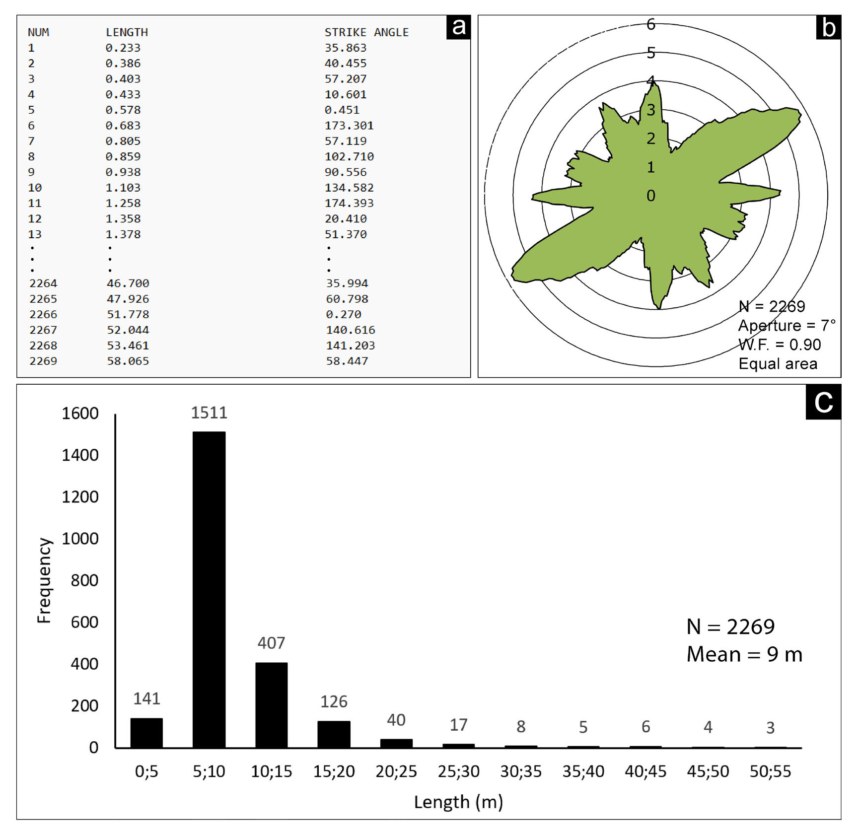
Using the “Fractures list” function, FA can scan the entire fracture dataset and derive the total number of fractures, their length, and azimuth with respect to the north (Fig. 6a). The total number of fractures documented in the Rosario Pavement is 2269 (Fig. 5). It varies in length between 0.23 m and 58.1 m, and the mean is 9.0 m. The analysis of orientations through the MARD (Fig. 6b) (Munro & Blenkisop, 2012) shows five fracture sets: Set1/N-S; Set2/E-W; Set3/NE-SW; Set4/NNW-SSE; Set5/WNW-ESE (Fig. 6b). The documented fracture sets are in agreement with Bagni et al. (2020) and references therein, where the set (N-S, E-W) originated from a regional stress field. The set (NE-SW, NNW-SSE, WNW-ESE) is a fold-related set of fractures. Set number 3 (NE-SW), being the most pervasive in the Rosario Pavement, controlled the development of Crotes Cave towards the NE-SW principal direction (Fig. 5). The length distribution graph (Fig. 6c) shows that most of the fractures, a total of 1511 fractures, are between 5 and 10 metres long. Conversely, due to the truncation effect, the fractures ascribed to the 0 to 5 m class are very few.
- Attributes of the fractures obtained with FA and its “fracture list” function (a). MARD (Munro & Blenkisop, 2012), n = 2269, aperture = 7°, weighting factor = 0.90 (b). Histogram of the distribution of fracture lengths every 5 m (c).
Scanline
Using FA’s “find scanline intersection” function, a linear scanline analysis of the fracture dataset is possible.
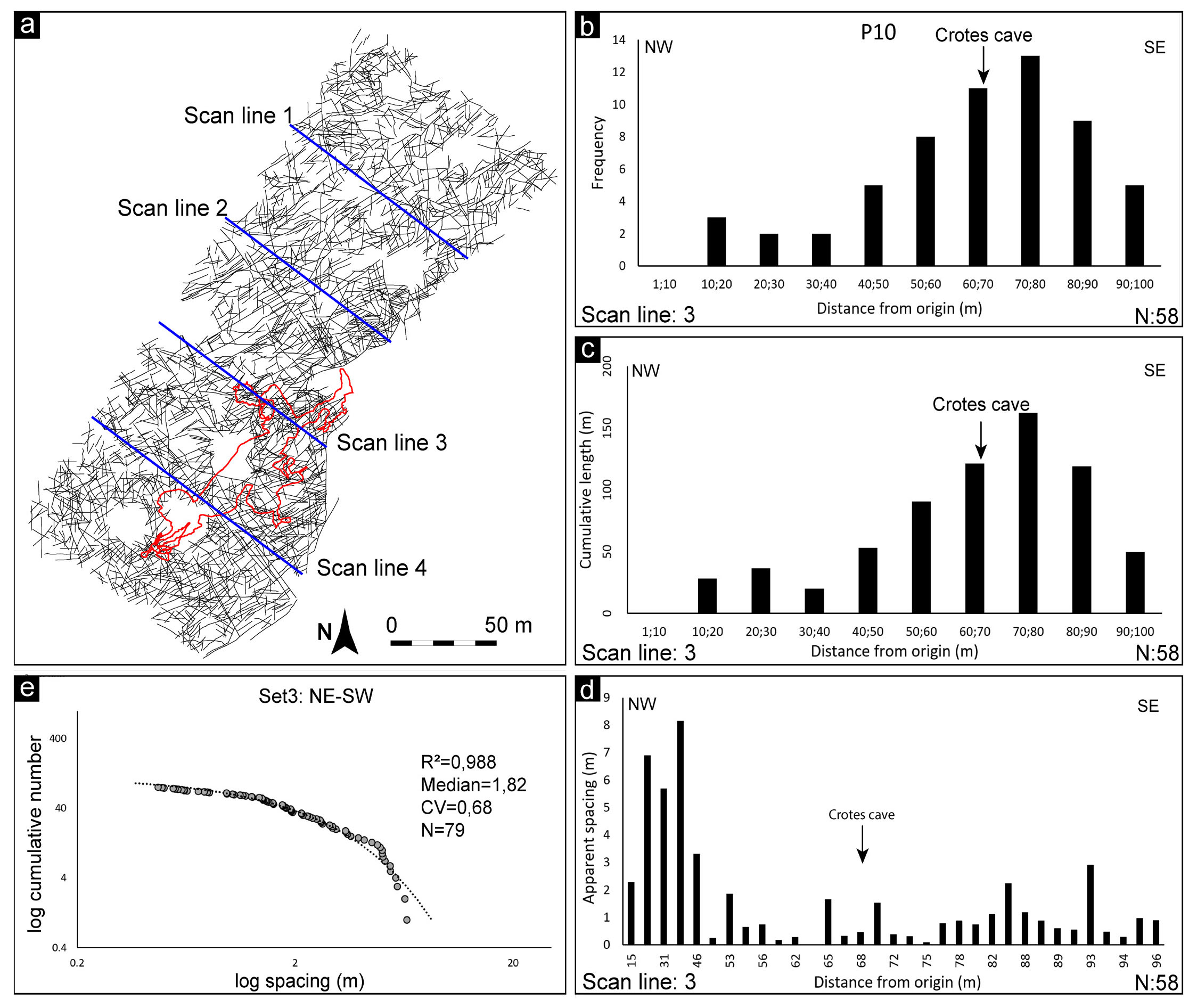
Four linear scanline analyses were performed on the Rosario pavement (Fig. 7a). The main trend of the scanlines is NW-SE. Hence, they are orthogonal to the axis of the Apodì fold, which is NE-SW. The fracture intensity distribution has been measured by moving away perpendicularly from the fold axis. The scanlines range in length from 95 m to 120 m and intersect 225 fractures. With the attributes derived by FA from the analysis of linear scanline number 3 (Fig. 7a), which is the most representative, it was possible to calculate other parameters indicative of the fracture distribution along the studied outcrop, such as P10 (fracture density) (Dershowitz & Herda, 1992) (Fig. 7b), cumulative length for unit length (Fig. 7c), and apparent spacing vs. distance graph (Fig. 7d). Furthermore, it was possible to calculate the log cumulative number vs log spacing plot concerning the fracture traces intersected by the four scanlines and belonging to the more pervasive NE-SW oriented fracture set (Fig. 7e). From the computed plots, it can be observed that P10 and cumulative length shows the same trend (Fig. 7b, c), so they gradually increase as above the Crotes cave (Fig. 7). However, a general increasing fracture trend approaching the Apodì fold axis is maintained (Fig. 7b, c). Moreover, the apparent spacing plot shows a decreasing trend as it approaches the axis of the Apodì fold (Fig. 7d). The analysis performed and presented in the plot of Fig. 7e shows an excellent match of the actual spacing data with an exponential regression line with coefficient of determination (R2=0,98), and coefficient of variation CV=0.68 that indicates an anti-clustered or diffused distribution of the fractures set (Sensu Giuffrida et al., 2019).
- Dataset of Rosario pavement and scanlines (a). Scanline 3 plots of P10 (b), cumulative length for unit length (c), and apparent spacing vs. distance (d). NE-SW fracture set attributes and relative log cumulative fractures vs log spacing plot (e).
Scan area
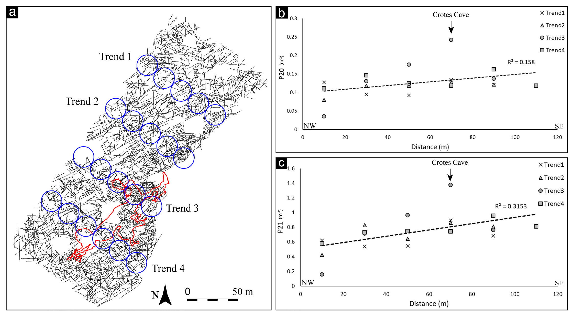
Scan area analysis with FA “compute scanarea density” function allowed us to automatically derive the values of P20 (fracture density) and P21 (fracture intensity) of the Rosario dataset and highlight the fracture trend distribution along the outcrop. A total of 21 scan areas with a diameter of 20 m were realised, organised along 4 NW-SE oriented trend directions (Fig. 8a), coinciding with the previous linear scanline analyses (Fig. 7a). The values of P20 resulting from the analyses vary between 0.04 m-2 and 0.24 m-2. In contrast, those of P21 vary between 0.18 m-1 and 1.37 m-1. The interpolated data with linear regression and coefficient of determination R2=0.158 for P20 and R2=0.315 for P21 show a gradual increase of P20 and P21 towards the SE, i.e., approaching the Apodi fold axis and displaying a clear peak above Crotes Cave (Fig. 8b). The maximum values of P20 and P21 were recorded along the trend 3 (Fig. 8b, and c) above the Crotes Cave and allowed rainwater to percolate and originate the Crotes cave (Bagni et al., 2020).
- Rosario dataset and scan areas (a). P20 plot (b) and P21 plot (c).
Fracture Spacing Index and Fracture Spacing Ratio analysis from Muggia sub-vertical dataset, Italy
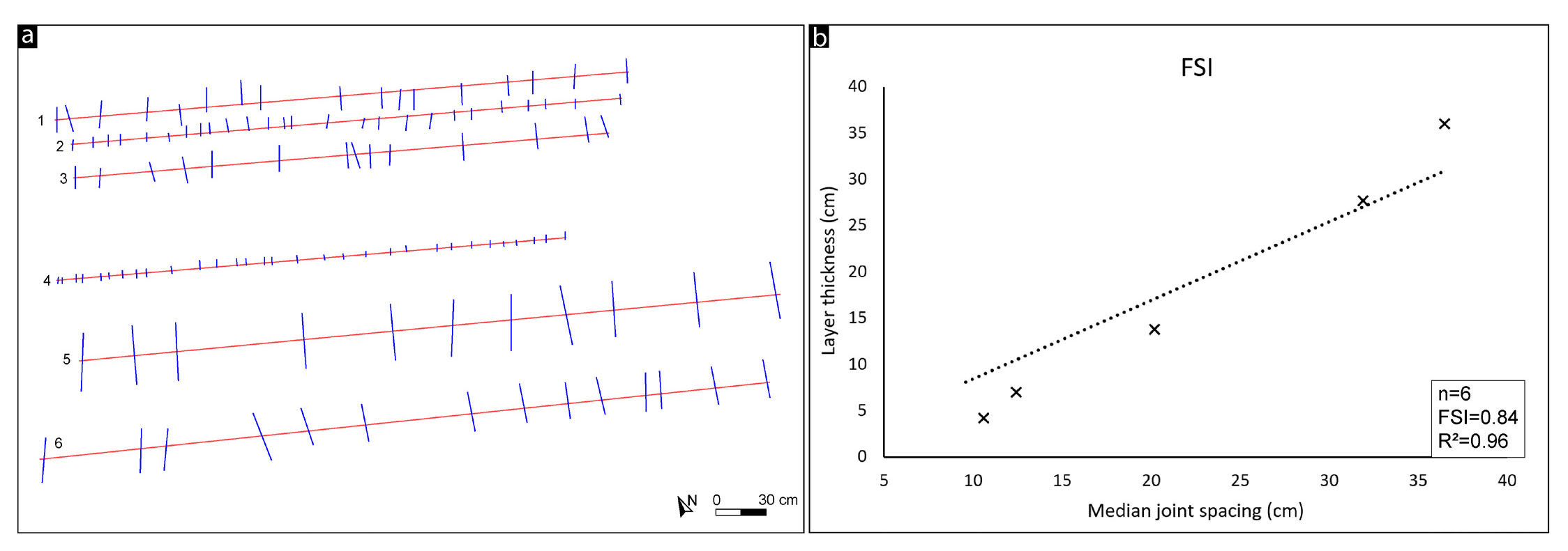
FA can use its ‘scanline’ function to investigate a sub-vertical outcrop and derive Fracture Spacing Ratio (FSR) and Fracture Spacing Index (FSI) values. Hence, six linear scanlines were performed in the sandstones of the Flysch of Trieste, intersecting a total of 113 fractures (Fig. 9a). Each scanline investigates an arenaceous layer of different thicknesses ranging between 7 cm and 36 cm. The median spacing between the joints varies from a minimum of 10.5 cm in scanline 4 to a maximum of 36.5 cm in scanline 5. Fig. 9b shows the FSR/FSI plot, where each cross represents the FSR value for each scanline, and the linear regression approximates the data well, with a coefficient of determination R2=0.96. The slope of the linear regression interpolating the various FSRs indicates an FSI=0.84.
- Muggia fractures dataset, where the blue lines are the fractures and the red lines are the scanlines (a); FSI (Fracture Spacing Index) plot, where the crosses are the FSR (Fracture Spacing Ratio) value for the scanlines (b).
CURRENT LIMITATIONS AND STRENGTHS OF FA
Limitations
FA assumes that the input fracture traces lie on a 2D surface and are orthogonal to the analysis plane. Currently, FA cannot process curvilinear fracture traces. In some cases, it is required to rectify the fracture traces, thus losing the true geometry and length. The azimuth angles of the fracture traces are measured in all directions but only reported from 0 to 180 in relation to the north. This limitation can be easily overcome by using bidirectional representations.
Strengths
A qualitative comparison was conducted between FA and other software to elucidate the primary innovations introduced by FA. The foremost distinction lies in the output format: while FA provides numerical results, the compared software delivers graphical outputs. Furthermore, FA organises its numerical data in a clear tabular format, with each row representing a fracture and its corresponding features arranged in columns. This structured data output facilitates subsequent analysis, such as filtering by orientation to isolate specific fracture sets. Another advantage of FA is its simplified scale management, as scale information is directly incorporated as a graphical element within the analysed file, contrasting with other software where it must be calculated and added separately. In the graphical output of the FA, fractures that were not processed due to geometric issues are highlighted, improving quality control. Regarding processing speed, FA outperforms other software in analysing large files (even exceeding 30,000 fractures) and delivering results within seconds, compared to other software with a minutes-long processing time. Additionally, FA offers distinct advantages over other software, including clear numerical output in scanline analysis and detailing the distance between fractures.
Moreover, FA is free-download and users can learn how to use it in a short time and, with just a few clicks and minimal knowledge of Python and graphics software, they can perform statistical analyses on the fractured state of a rock mass outcrop, a scanned thin section, orthoimages or on any other digital picture as shown in Fig. 10. The Python script starts automatically, and the clear user interface (Fig. 1a) allows for the easy selection of the desired analysis function. FA can currently perform a complete fracture density and intensity analysis of a wall or pavement outcrops in 1D and 2D, calculating the P10, P20, and P21, as described in Dershowitz & Herda (1992). Currently, FA has no limit on the number of data and orders of magnitude that can be analysed, the only limit being the memory and computing power of the computer used.
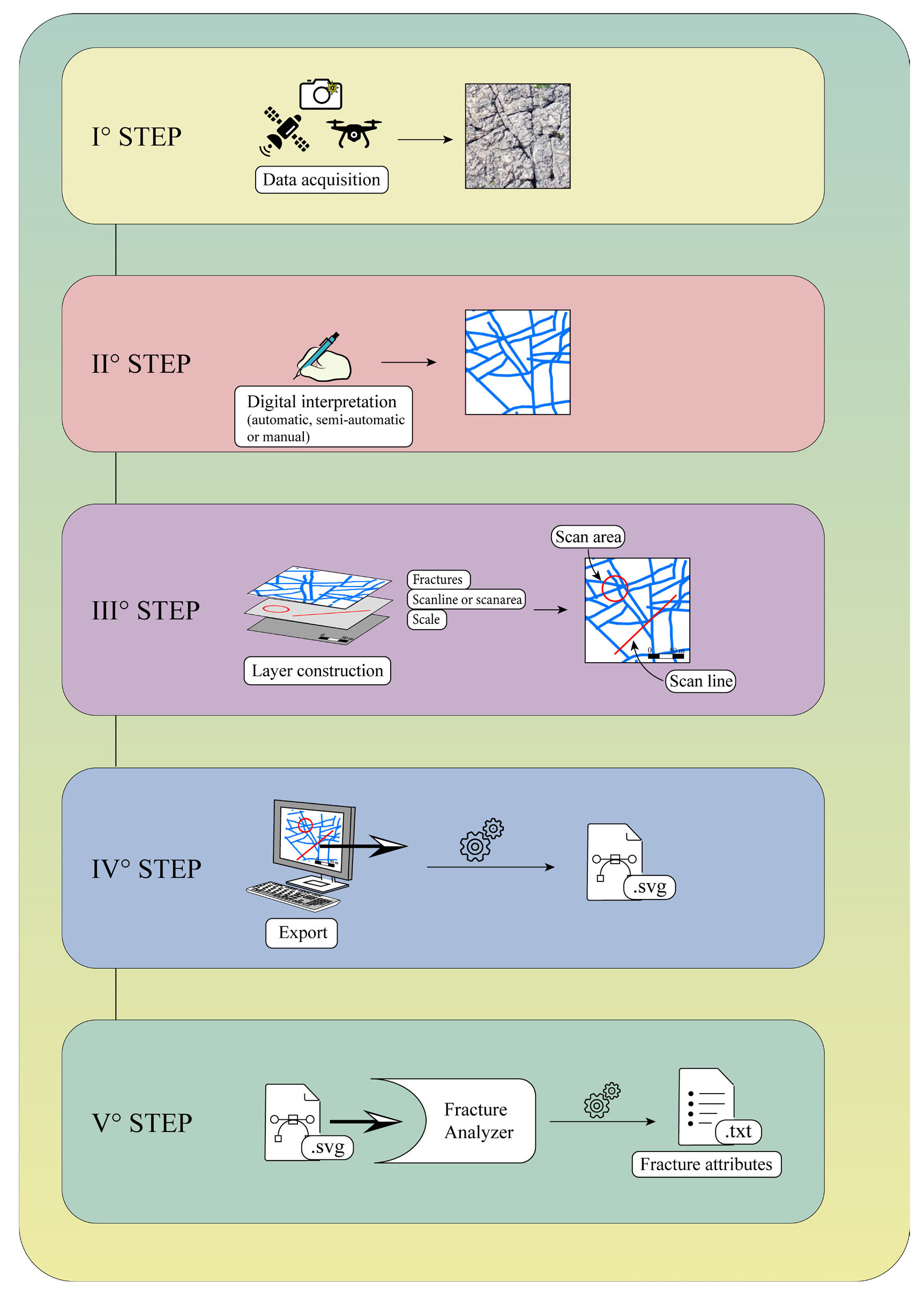
- The concluding diagram of the operation of FA is divided into five steps.
CONCLUSION
This paper describes Fracture Analyser (FA), a new software-based toolbox for quantifying fracture patterns in 2D. The tools in the software provide an objective method for analysing, starting from a vector graphic file (.SVG), a dataset of fractures from a wide range of scales, rock types, and structural settings. The proposed method has never been presented with such an easy and intuitive application (Fig. 10). We have shown how FA can quantify fracture patterns on pavement outcrops or sub-vertical outcrops without any scale limitations. The FA obtained fracture attributes pattern dataset allows users to systematically quantify statistical and spatial variation and compare different areas and scales.
The examples presented in this paper demonstrate that geologists can use FA to derive fracture attributes from a dataset, objectively and repeatable, to quantify the fracture state of an outcrop and compare it with other locations. A 2D linear and areal method of fracture patterns density and intensity estimate is provided to obtain an objective parameter that can be compared with other fractured areas in other tectonic contexts.
The toolbox has been developed in Python. The source code is public so other developer users can implement other fracture analysis functions.